GIS 1 Lab 4

Goals and Background:

The goal of this lab was to use the skills I learned from lectures and tutorials in class to develop queries that returned the desired results in the instructions and assess my knowledge of attribute queries and spatial queries. A combination of Boolean expressions, operators and parentheses were used to develop the correct multiple criteria queries that the instructions requested.

Part 1

Query 1

Methodology:

Part one focused on the United States for building multiple criteria queries. From a blank map in ArcMap I added the counties shapefile from the USA geodatabase in my mgisdata folder. To begin building my first query I opened the selection drop-down menu from ArcMap and chose the 'Select by Attributes' tool. This opened a new window in which I chose my layer to select attributes from, in this case counties. The method of choosing the attributes remained at its default 'Create a new selection'. The next step was to begin building query 1 and to do so I first added parentheses to my query to separate one part from the other, then I scrolled through my options until I found the expression that represented the 2010 population 'POP2010'. Double clicking on the expression added it to the query box. In order to get a result that returned a population between 3000 and 4000 I added a greater than or equal to sign to include 3000, then I added the AND operator to include all attributes between the two numeric values: 3000 and 4000 and selected 'POP2010', a less than or equal to sign and entered in 4000 as the final numeric value in this part of the query. Another parenthesis closed off the first part so I could begin on the second part of query 1. The second part was left out of parentheses because they were not necessary as the first part was already separated from the second part. The second part of query 1 required the use of a new Boolean expression "POP10_SQMI. This expression would return results of the 2010 population in persons per square mile and for this particular part of the query, I wanted the population per square mile greater than or equal to 1000. First I had to use an OR operator, this operator selects records for which either expression is true, that is it would select records that have a population between 3000 and 4000 and it would select records that have a population per square mile over 1000. After the OR operator I added the 'POP_SQMI' expression, the greater than or equal to sign and 1000 as the final numeric value. In order to execute the query to actually return any records, I first verified it to check for any errors and then clicked okay. The counties highlighted were the records returned from the query. From the counties layer in the Table of Contents, I right-clicked it to open a new menu and under the selection tab I chose to create a new layer from the selected attributes. This created a  new layer so I could create a cartographically pleasing map instead of having all of the selected counties outlined by the query.

Query 1: Multiple criteria query that shows counties with a population between 3000 and 4000 people in 2010 as well as counties in 2010 that had a population density greater than or equal to 1000 persons per square mile.  

Query 1 results

Results:

The results from query 1 are shown above. The query I developed was a multiple criteria query that returned counties in the United States with a population between 3000 and 4000 (including 3000 and 4000) and counties that had a 2010 population density of at least 1000 persons per square mile.  The resulting query and map are shown above with the desired counties highlighted in yellow on the map.

Query 2

Methodology:

Query 2 focused again on the United States when returning desired records. I began first by clearing the first query from the map and from the select by attributes window. The first step to creating Query 2 was similar to Query 1 in that I used the selection tool to open the select by attributes window. The layer stayed the same, counties and the method also stayed the same, create a new selection. For this query I wanted counties within specific states so to start the query I needed to specify which state I wanted. To do so I entered the expression 'STATE_NAME', an equal sign to indicate the exact state I wanted results from and the state name. After I used the AND operator to isolate specific results within that state. To follow that I added parentheses to separate one part of the query from the other, and in the parentheses I added the male population greater than the female population. The last part of the query, followed by another AND operator was intended to return results of counties with a senior population greater than 6500. to add this to Query 2 I found the 'AGE_65_UP' expression, added a greater than sign and added the 6500 value.

Query 2: Multiple criteria query that shows counties in Wisconsin where the male population is greater than the female population and where the population of seniors (ages  65 and up) is greater than 6500. Other queries were created with the same structure but for different states: Texas, New York, Minnesota and California.



Query 2 results

Results: The query I developed was a multiple criteria query that returns counties in a state that have a male population that is greater than the female population and counties that have a senior population, ages 65 and up, that is greater than 6500. The states I used for this query were Wisconsin, Minnesota, California, Texas and New York, the counties in each state are highlighted in different colors: Wisconsin counties in orange, Minnesota counties in purple, California counties in pink, Texas counties in yellow and New York counties in green.

Query 3

Methodology:

Similar to the first two queries, Query 3 focused on the United States counties. From the select by attributes window, the layer remained on counties and the method remained on create a new selection. I also maintained the use of the 'STATE_NAME' expression, as I wanted results from specific states. The query begins by naming the state I wanted to isolate then using the AND operator to separate the first part of the query from the second part. Parentheses were also used for the second part to further isolate that specific part of the query from the first and third parts. After the AND operator I added the parentheses and within those I added the 'AGE_65_UP' expression followed by the greater than sign and 6500 as a numeric value. I ended that part of the query with a closing parenthesis and another AND operator to indicate a new part of the query. The final part made use of the 'HSE_UNITS' expression which indicates the number of housing units per county. After this expression I added a greater than sign and 30000 as a numeric value.

Query 3: Multiple criteria query that shows the counties in a state containing seniors ages 65 and above and containing more than 30,000 housing units. The same structure of the query was used for multiple other states, including Washington, Maryland, Illinois, Nebraska and District of Columbia.

Query 3 results

Results: The query I developed was a multiple criteria query similar to the first two. This query returned results for counties in the states of Washington, Maryland, Illinois, Nebraska, District of Columbia and Michigan. The query intended on returning results for counties where the senior population was greater than 6500 and those counties also contained more than 30000 housing units. Washington counties are shown in dark orange, Illinois counties are shown in pink, Michigan counties in yellow, Nebraska counties (though very few) are shown in a pale orange, Maryland counties in green and unfortunately, the District of Columbia counties were too small to be seen on the map.

Part 2

Query 1

Methodology:

This query had multiple parts using two different tools. I started by using the select by attributes tool and entered in the query " 'POP2007' > 15000 AND 'POP2007' < 20000 AND 'AREALAND' >= 5 AND 'FEMALES' > 'MALES' " This part of the query was separated by the AND operators So it would return population data, city area data and the ratio of females population greater than the male population. After applying that part of the query I opened the select by location tool and changed the selection method to "select from the currently selected features in". This would ensure that the results returned from this part of the query stemmed from the first part. I chose the target layer as WI_cities, the source later to be Lakes, and the spatial section method to be "are within a distance of the source layer" with a distance of 2 miles. Finally, I clicked the OK button to apply this part of my query to the first part.

Query 1: Selecting by both attributes and location to return a result of the cities in Wisconsin that have a population between 15,000 and 20,000, where the female population is greater than the male population, the area of the city is greater than or equal to 5 square miles and the city is within 2 miles of a lake.

Query 1 result

Results: The results of Query 1 returned data of cities in Wisconsin that have a population between 15000 and 20000, with a female population greater than the male population and the area of those cities being greater than or equal to 5 square miles. This was part one of Query 1. Part two of Query 1 was a location query that returned results of the cities selected in part one that were within 2 miles of a lake. A map of the results and the two queries are shown above

Query 2

Methodology:

This query was simple to construct but involved selecting multiple rivers. To do so I simply added the 'PNAME' expression an equal sign, and the name of the river I wanted to select. To include other rivers in the same selection I would add the AND operator and use the same structure as the first part of the query: 'PNAME' = "river name". I got the river names from the unique values list to save time instead of typing out all the names.

Query 2: The same structure was used for different rivers listed.

Query 2 result

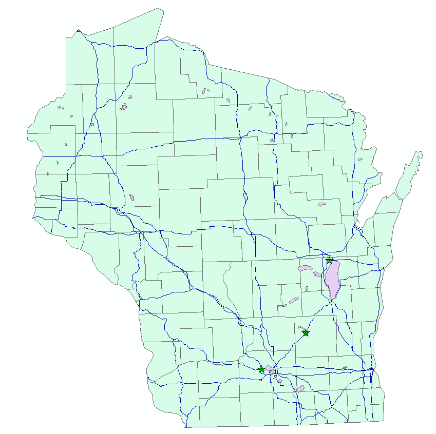
Results: The results returned a record of the rivers I selected from the instructions given to me. In the map above the results are shown with a backdrop of major roads, lakes and counties in Wisconsin. The rivers selected are: The Chippewa River, Eau Claire River, Embarrass River, Fisher River, Hunting River, Kinnickinnic River, Maunesha River, Milwaukee River, Moose River, Namekagon River, Pelican River, Platte River and Potato River.


GIS Lab 3

Lab 3 technical report

Goal and background:

The goal of this lab was to create a static map and a dynamic map of the state of Wisconsin. The static map includes information about the population per county, and a variable of my own choosing, in this case the number of housing units per county. All of the data contained within the static map was derived from the U.S Census Bureau as part of their 2010 Census data. The dynamic map was produced online, through the ArcGIS website, and serves as a way of sharing the information I obtained pertaining to the number of housing units per county in the state of Wisconsin.

Methodology:

 To begin building the static map, containing two data frames for the population and housing units of Wisconsin, I went to the US Census Bureau website. From there I chose an advanced search and narrowed my selections down to the total population of Wisconsin by choosing “2010 SF1 100% Data” as my topic, “County” as my Geography, “Wisconsin” as my state and “All Counties Within Wisconsin” to ensure I would obtain data on all Wisconsin counties. From there I found the “Total Population variable and downloaded it to my lab 3 folder. The download came in as a zip file, so unzipping it was necessary to obtain the CSV files needed for my maps. The P1 table contained in one of the CSV files I needed would not be compatible with ArcMap if I left it as is, so I saved it as a MS Excel file instead by changing the file type from the save as tab as Excel Workbook.

The next step was to download the shapefile of Wisconsin from the Wisconsin Census data. From the Geographies tab, I clicked on the map tab to show the state of Wisconsin highlighted since that was what the data I had chosen previously pertained to. I downloaded the file to my lab 3 folder and formatted it to a shapefile so it would display on my map correctly. This file also came in as a zip file so unzipping it was necessary as well.

Finally I was able to start building my maps, now that I had all the necessary components for the population portion. I connected ArcMap to my lab 3 folder and added the Wisconsin shapefile and the P1 table to my blank map. The next task was to join a standalone table and an attribute table. In this case, the standalone table was the P1 table and the attribute table was the Wisconsin shapefile table. I right-clicked on the shapefile in my table of contents and highlighted the joins and relates tab, a sidebar opened and from there I chose join. A join window opened and the field I based my join off of was the GEO ID field because both the standalone and the attribute table had this field. Next I chose the table to join to the shapefile table, in this case, the P1 table and the field in that table to base the join on was the same, GEO ID. Then I validated the join and clicked OK. This joined table needed to be displayed as its own shapefile so I exported the data by right-clicking on the Wisconsin shapefile feature and pointing to Data and then Export Data. Then I saved the data as a shapefile with a name of my own choosing and the new shapefile of Wisconsin was displayed on my map.

The next task was representing the attribute table on the map. To do this I opened the properties for the new Wisconsin shapefile and chose the symbology tab. Since the value I needed, D001, was a set as a string type I had to go back into the attribute table, create a new field which I named “newD001” and added the same data from the D001 field using the field calculator and saving it as a long integer type instead of string type. Then I went back to the symbology tab and chose D001 as my value in the graduated colors section under quantities.

The first part of my static map was finished, containing the population of Wisconsin by county. The next map required me to make a map of a variable of my own choosing, in this case I chose to make a map of the number of housing units per county in Wisconsin. This procedure followed the exact same steps as the previous map. I downloaded and unzipped the census data from the US Census Bureau website and converted the desired CSV file to an Excel file, added it to the new data frame on the same map along with the original Wisconsin county shapefile and joined the standalone Excel table to the shapefile table. I then exported the data as a new shapefile and changed the symbology accordingly for the new map.

Next was designing the layouts for the finished maps. This required a change in projection more appropriate for the state of Wisconsin and in this case I chose to do a NAD 1983 Wisconsin Transverse Mercator projection. To do this I opened the data frame properties for both frames, clicked on the coordinates tab and changed the projection to NAD 1983 Wisconsin TM (Meters). Next was an addition of a title, legend, north arrow, scale bar, date, source and my name as the author of the map. All of these could be found in the insert tab, under their corresponding names. Finally I simply had to move and scale everything so the map looked organized and appealing.

Part two of lab 3 involved creating a dynamic map displaying the data derived from the static map.  For this part I used the map containing my variable choice, housing units. To begin, I removed the population data frame from the map document, leaving the housing map. From ArcMap  I signed into my ArcGIS online account that’s through UW-Eau Claire so I would be able to share my map with the UW-Eau Claire geography department. Since dynamic maps are online, and I needed to share my map online, I needed to create a feature service for my map. To do this I clicked the file drop-down menu and chose the share as tab. A sidebar appeared giving me two choices: “Map package” and “Service., I chose service. A new window opened up that would take me through the share as service process. In the first window I chose to publish my map as a service, then clicked next. The next step was to choose where to publish my service and a drop-down menu appeared giving me the choice to publish my service to “My Hosted Services” in this case UW-Eau Claire Geography and Anthropology. Below it I created the name for my service and clicked continue.

The next window to open was the service editor window, this allowed me to choose the capabilities of my map, give it a description, a summary and tags and allowed me to choose who I was sharing my service with. Finally, I clicked analyze and a pop-up window appeared showing me any warnings or errors that appeared. I resolved any errors I had and clicked the publish button to publish my service. Once the publishing was complete I signed in to the ArcGIS website and viewed my service under the contents page. The last thing I needed to do before I saved and shared my map was edit the data that could be viewed by clicking on each county. I found the feature layer of my service and clicked the arrow to display a drop-down menu and from there I chose “add layer to map”. This displayed my map of Wisconsin over a base map of the U.S. Since I only needed two attributes to be shown, county and number of housing units, I clicked on the content button to the left side of my map and clicked on the three dots underneath my service name to expand a menu. In that menu I chose the “Configure Pop-Up” option that opened a window allowing me to select what attributes are being displayed on the map and what their names are. I chose the “NAME” attribute, and the attribute for my housing units labeled “newD001”. I renamed them “County” and “Housing Units”. I then clicked OK to save the changes and clicked the “Save Pop-Up” button near the bottom of the window.

The last step to completing part 2 was to save and share my map. First I saved my map by clicking the save button near the top of the page and chose the “save” option. This opened a new window allowing me to enter a title, tags and a summary for my map and where to save my map. Once all the information was entered correctly I clicked the “Save Map” button. Lastly I needed to share my map and to do so I went to my content page and clicked on the name of my web map to open its properties. From there I clicked the share button which opened a new window in which I checked the UW-Eau Claire- Geography and Anthropology box. This allowed me to share my map with that specific group.

Results:

The results I obtained were 2 maps, one static and one dynamic that displayed the skills I acquired from this lab and previous labs and tutorials. One map is the static map of the state of Wisconsin, showing housing units in the top data frame and population in the bottom data frame. Each data frame has its own legend, scale bar and north arrow. The dynamic map is a screenshot I took of the final product of my published service in the form of a web map. It shows the housing units data frame from the static map over a base map of the U.S. This map is displaying the number of housing units in each county, with an example being shown of 23,996 housing units in Door County.

Dynamic Map

Static Map

Credits: US Census Bureau (2000). American FactFinder . Retrieved from http://factfinder2.census.gov/faces/nav/jsf/pages/index.xhtml

GIS 1 Lab 1

Goal and Background:

• The goal of this lab is to become familiar with projected coordinate systems and geographic coordinate systems. Through this lab I have learned the difference between the two, and which projections are the appropriate ones to use based on the data displayed on the map. For example, the Wisconsin map I created has a North America 1983 geographic coordinate system. This coordinate system was chosen based on information from the metadata provided to me from the Lab 1 instructions. Following that, I chose a North American 1983 StatePlane projection with a Central Wisconsin focus as the projected coordinate system because the GIS data displayed on the map portrayed the Central Wisconsin area. These coordinate systems did not come with the shapefiles, so I had to use one of the other skills I learned from this lab and previous tutorials to adjust the projected coordinate systems to the appropriate ones so that the display of the data on the map would be accurate. Through this lab I was able to detect and resolve any projection errors within the GIS data.

Method:

•  Every new map that is opened in the ArcMap starts out as blank and all of the data I used in this lab was taken from the Lab 1 Data folder I obtained from my instructor, this folder contains several subfolders that store the data needed for this lab. The first step I took was adding two shapefiles from the World folder to get a map of the world with the geogrids shapefile displayed behind it. The next step was implementing the skills I learned from previous tutorials to adjust the geographic coordinate system to WGS 1984. This final step was the last one to complete my first data frame, labeled “Geographic Projection”. To do this I found the coordinate systems tab under properties of the Geographic Projection frame and from there I found the WGS 1984 projection under the World subfolder of the Geographic Coordinate System folder.  Similar steps were taken for the next four data frames, each with its own individual projected coordinate system: Mercator, Sinusoidal, Equidistant Conic, and Robinson. Each of these projections can be found under the World subfolder of the Projected Coordinate Systems folder.
                  The next portion of this assignment asked me to work with projections at a state level, as opposed to a world level like in the previous section. This part of lab 1 began with a shapefile of the United States from the USA folder. From there I had to isolate the state of Wisconsin from the rest of the map, in order to create an entirely new shapefile of Wisconsin alone. To do so, I opened the Select by Attributes tool and entered the “STATE_NAME” = “Wisconsin” clause to isolate Wisconsin. I then created a layer from the selected features and exported those features to my lab data folder as a new shapefile for Wisconsin. After changing the projection to the “UTM, NAD 1983, Zone 16N” projection by finding the UTM folder under Projected Coordinate System, opening it to the NAD 1983 folder and selecting NAD 1983 UTM Zone 16, I had my sixth data frame completed.
                  My seventh and final frame was a map of the United States that showed the roads that ran throughout the state of Michigan. A states shapefile and a Michigan state roads feature were added to the final data frame. The problem with this map was that the two features lined up correctly, but it was in an on-the-fly projection, meaning that certain types of analysis would not be possible with just this type of projection. That being said, I needed to change the projection of the Michigan state roads feature. To do so, I opened ArcToolbox then under the Data Management Tools I selected Projections and Transformations and then the Project tool. This allowed me to give the shapefile a different projection, without changing the geographic coordinate system. I input the Michigan feature then, I changed the output coordinate system. I found the Layers folder, and underneath it was a GCS_North_America_1983 category. I expanded that and found the states shapefile, and selected this to change the projection of the Michigan feature to match the projection of the states shapefile. Finally I assembled all of the data frames on one map and organized them as seen in Figure 1 below.

  

  Figure 1: Maps and their projections

                  The final portion of this project required me to resolve projection problems between two features being projected on the same map. The first was a shapefile I added of Central Wisconsin counties. This shapefile had an undefined geographic coordinate system. This meant that I needed to choose a geographic coordinate system for this shapefile. Based on the information from the metadata that was provided to me in the lab 1 instructions, the geographic coordinate system I gave this shapefile was North America 1983, or NAD 1983. To do this, I opened ArcToolbox, and under the Data Management Tools I selected Projections and Transformations and then Define Projection. I selected the counties shapefile and the geographic coordinate system I wanted and clicked OK to define the projection.  

  

  Figure 2: Map of Central Wisconsin Counties and Rivers

                  The next step was to add the rivers polyline feature from my lab data. This shapefile brought up another issue because the projection of this shapefile was not the same as the projection of the counties shapefile. Both projections need to be the same in order for the map to be displayed accurately. To solve this problem I went back to ArcToolbox and instead of choosing the Define Projection tool I chose the Project tool. I input each feature separately into the tool and selected the desired output, this being a North American 1983 StatePlane projection of Central Wisconsin. Clicking OK created a two new features to replace the old features on the map. I removed the old counties shapefile and the old rivers polyline and I was left with an accurate map of Central Wisconsin counties and the rivers that run through them.

Results:

• The results of the maps (Figures 1 and 2) and my methods reflect my understanding and ability to resolve issues related to geographic and projected coordinate systems.

Sources:

• Michigan Department of Transportation. (2016). Retrieved from michigan.gov/mdot.
• Maribeth Price. (2016). Retrieved from Mastering ArcGIS and mgisdata.